Introduction and Notations

This page introduces two methods for assessing sensitivity to unmeasured confounding in marginal structural model (Matteo, Edward, Valérie, and Larry, 2022). Recall that we have 3 usual assumptions in MSM: consistency (No interference), Positivity (Overlap), and Sequential Exchangeability (No unmeasured confounding). In the previous discussions, we knew the treatment is as good as randomized within covariates. That means there are no unmeasured variables that affect assignments and outcomes. Because the first two assumptions are not easy to be investigated, we will do sensitivity analysis on the third assumption.

Suppose our data are n iid observations . Note that X represents covariates, A means assignments (treatments), and Y is a vector of outcomes. To easily do the sensitivity analysis, we simplify our MSM model. The first step is to rewrite our model into the form of linear model. Let the causal mean

be a model for the expected outcome under treatment assignment . An example is the linear model for some specified vector of basis functions . It can be shown that in previous expectation satisfies the k-dimensional system of equations

for any vector of functions , where can be taken to be either IPTW or the combination of IPTW and IPCW. Furthermore, we estimate by solving the above expectation which leads:

In the next section, we discuss the first step of our main topic: Sensitivity Models.

Sensitivity Models

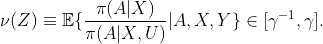
In this section, we introduce two models for representing unmeasured confounding when treatments are continuous. Each model defines a class of distributions for , where U represents unobserved confounders. Note that our goal is to find bounds on causal quantities, such as or .

1. Propensity Sensitivity Model

Consider A is continuous, we apply density ratios rather than odds ratio model to define our model:

To interpret the model, we can see it as defining a neighborhood around .

2. Outcome Sensitivity Model

For this model, we define a neighborhood around given by

which is a set of unobserved outcome regressions, , such that differences between unobserved and observed regression differ by at most after averaging over measured and unmeasured covariates. Based on above model, we immediately obtain the simple nonparametric bound .

In the next two sections, we present bounds on these two different models, respectively.

Bounds under Propensity Sensitivity Model

A preliminary step in deriving bounds for the MSM is to first bound where and

It is easy to see that . So bounding is equivalent to bounding .

Combining the above findings and Lemma 1, 2 in (Matteo, Edward, Valérie, and Larry, 2022), we have that if . This implies that . When the MSM is linear, we finally obtain

See details in section 4.3 (Matteo, Edward, Valérie, and Larry, 2022).

Bounds under the Outcome Sensitivity Model

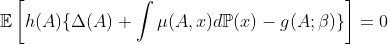
Considering the outcome sensitivity model, we obtain

We can write a corresponding MSM moment condition as

Then, it is straightforward to estimate by solving the empirical, influence function based, bias-cprrected analogs of the moment conditions

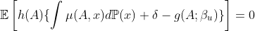
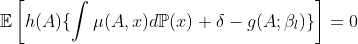
In the linear MSM case, we can rewrite our bounds based on similar concepts as proepnsity sensitivity model. And, we finally obtain estimators

See details in section 5 (Matteo, Edward, Valérie, and Larry, 2022).