
Set up: simplification
Before we discuss our identification, we need to simplify our scenario as the following DAG :
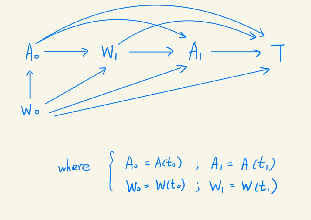
and notations (corresponding to Casual Inference 1).
To interpret identification easily, we simplify our scenario at first. Next, we introduce the assumptions.
Assumptions
We need the following set of assumptions to identify causal effect:
- Consistency (if A=a, then T=T(a) for all a)
- Positivity (0 < P(A=a | W) almost everywhere, for all a)
- Sequential exchangeability
We need sequential exchangeability rather than conditional exchangeability, because conditional exchangeability is always violated in time-varying data. Sequential exchangeability includes two conditions:
- (C1)

- (C2)

The covariates that satisfy (C2) through their stratification are called time-varying confounders. The three assumptions are general in most topics of causal inference, because we cannot observe potential outcomes in our universe.
Identify Causal Effect
Under our three assumptions, the g-formula is equivalent to the averages of potential outcome. If baseline confounders Wo exist, we obtain the following equation by g-formula:
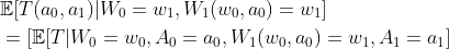
Summing,
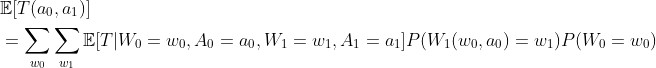
Then we use g-formula again,

Thus, our result is

To interpret our result, it is easy to know that our survival time T is based on time-varying treatments A, which are affected by time-varying confounders W. Besides, W is also affected by previous A. Note that we only considering 2 states then obtain such the complicated structure. If we consider K states, the structure is too complicated to calculate (we will show it later). Thus, it also motivates us to find out more efficient way to assess the effect of treatments to survival time. That’s why our proposed method is Marginal Structural Model.
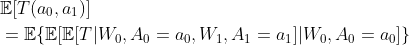
Also, we can show a representation of the iterative conditional expectation of the g-formula. Starting from our result, according to the definition of expectation, we obtain:

Then, by the definition of conditional expectation:
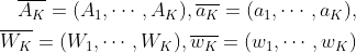
Finally, we can generalize our results into fixed K states:

,where
The notorious structure motivates us to find another method to reach our goal.
Inverse Probability Weighting
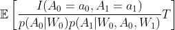
The alternative expression of ![]() under (C1) and (C2) is inverse probability weighting:
under (C1) and (C2) is inverse probability weighting:
Until now, we have two ways to identify our causal effect; however, our interest is in modeling Cox-type survival model. We will go back to our Marginal Structural Model in the next section.
Previous section: Causal Inference 1 – Introduction
References
- Shinozaki T, Suzuki E. Understanding Marginal Structural Models for Time-Varying Exposures: Pitfalls and Tips. J Epidemiol. 2020 Sep 5;30(9):377-389. doi: 10.2188/jea.JE20200226. Epub 2020 Jul 18. PMID: 32684529; PMCID: PMC7429147.

Leave a comment